Math Movement

Tomorrow, Harry Potter and the Deathly Hallows – Part 2 opens around the country. It is also the day I return to Charlotte from the Yale National Initiative’s Intensive Session. In honor of a successful week at Yale and what will undoubtedly be a successful opening day for a movie, this blog entry is inspired by a Yale National Initiative seminar that can uncover the trick behind the apparent magic in the YouTube movie below:

Yesterday, I visited the seminar Great Ideas of Primary Mathematics led by Roger E. Howe and Amanda Folsom. A technique taught in the session was the use of a table to deepen the understanding of multiplication. For instance, suppose we multiplied 21 by 13. Then, we form the table:

	10	3
20
1

Then, each entry of the table is filled with the product of the numbers in its respective row and column, as seen below.

	10	3
20	200	60
1	10	3

Now, to simplify the discussion below, let’s concentrate only on the entries that we were products of row and column headers in the table above. This gives us:

200	60
10	3

Adding the entries of the table gives the desired product to our problem, 273. However, notice for a moment that we could also add along the 3 diagonals that run from the upper right to the lower left. Our first diagonal has only one entry 200. The second diagonal has the numbers 60 and 10; so the sum is 70. Finally, the last diagonal has the entry 3. As you sum along each diagonal, the numbers have the same place value. The first is hundreds, the second tens and the last ones.

Let’s use this knowledge to look at the trick again. Below is my rendering of the trick with the intersection points delineated by color.

Compare this to the table and adding along those diagonals. Notice a similarity? If not, the colors of the dots may help. Each color corresponds to a different place value. Each purple dot is a hundred, each green ten and each orange one. Further, notice how adding the dots, particularly in the middle of this picture, corresponds to adding along the diagonals in the table.

Got it? Try the method of drawing lines to find the product of 32 and 12. When you get that, try 62 times 14. You might want to go back to the table, if you struggle to think through what to do with the sums you get with the points.

Magical? Indeed, at least for mathematical Muggles!

I compose this blog while stretched out on a dorm bed at Yale University. I’m midway through my time at the Yale National Initiative’s Intensive Session as a College Faculty Member given my involvement with the Charlotte Teachers Institute. My time has been inspiring and thought-provoking.

Today, I visited the seminar Great Ideas of Primary Mathematics led by Roger E. Howe and Amanda Folsom. Michael Pillsbury, the seminar coordinator for the CTI seminar Math through Pop Culture that I lead, is a national fellow and creating a curriculum unit from the ideas of Howe and Folsom’s seminar. This week has afforded us wonderful opportunities to discuss mathematics and innovative ways to encourage students to delve deeper or broader into their knowledge of content.

Yesterday, Mike showed me an interesting variation on subtraction that connects to discussions that subtraction is the addition of positive and negative numbers. Let’s consider subtracting 359 from 746. First, we line the numbers up as we probably did in grammar school:

With the standard algorithm, we would borrow to get:

Such a method calls for an understanding or at least makes mechanical use of place value as we “borrow”. Consider Mike’s approach that calls for the use of negative numbers. This technique caught my eye and had me thinking about subtraction in a way that pulled me from my usual mechanical response to a problem.

Now, simply add the numbers along the bottom row to get 400 + (-10) + (-3) = 390 – 3 = 387. Such a method sheds a different light on the method of subtraction and depending on your student’s outlook and mathematical preferences, might be most helpful.

Thanks to Mike Pillsbury of Randolph IB Middle School. If only I could infuse this blog post with the laughter and joy that comes naturally when learning it with him!

A clever use of mathematics can mystify audiences. A variety of resources divulge such secrets for a budding mathematically-inclined magician. Colm Mulcahy’s (Spelman College) column Card Colm on MAA Online reveals the mathematics behind a variety of tricks that involve such topics as Fibonacci numbers and results of Paul Erdös.
Mathemagician Art Benjamin (Harvey Mudd College) unveils secrets of rapid mental calculation in his book, Secrets of Mental Math. How magical such tricks appear is correlated to one’s insight into the underlying mathematics.

Last week, I started following Colm on Twitter at @cardcolm and began wondering about YouTube videos on math-based card magic. I quickly bumped into this one:

As evident in the video, and soon verified with a deck of cards in my office, the trick does not rely on any specific ordering. As I reflected on the mathematics behind the magic, I noticed, of course, that the trick relies on placing the chosen card ninth from the bottom. There are 52 cards so the chosen card is 43 from the top. Initially, this seemed one card off. However, then I imagined capping all 4 piles. In this case, the last pile IS capped with the chosen card. However, in every other case, the trick works the same way. You sum the cards that are face up and count that many cards down. If the sum is 10, for example, the tenth card is the chosen card. Why does the trick work? I’m going to leave that to your mathematical exploration, mainly due to my repeated inability at writing a clear, succinct answer.

Unless you cap all four piles, you are able to add up the sum of the cards that are face up and count that many cards down to unveil the chosen card. If you cap all four piles, there are no cards face up. In such a case, the “zero” card (rather than the first or thirteenth card, for instance) is the chosen card. Granted, a magician, such as yourself, could finesse unveiling such a “zero card,” which would be the card to cap the fourth pile. In my mind, this is less magical than counting down and finding the chosen card. I found myself wondering, “What is the probability of this even happening?” Feeling quite nerdy but not minding (much), I grabbed a pencil and paper and begin trying to compute such a probability. Soon, it appeared I would need to cover several cases or sit until I perceived another approach. Then, I laughed in the realization, “I’m a mathematician and computer scientist! Let the computer do the computing!”

I quickly coded a MATLAB program to perform the trick. I created a deck and randomly permuted the cards to serve as my shuffle. Then, I simply performed the trick 100,000 times keeping track of how often I capped all four piles in the trick. The first time I ran the computation, this occurred 1352 times. The second time I (via MATLAB) performed the trick 100,000 times capping all four piles 1336 times.

So, I would have about a 1.3% chance of this happening! Given I rarely perform magic, this is a pretty small chance. If I decided to perform the trick more often, could I live with that probability? Would you? It may partially depend on what you do when the case arises. Frankly, I might just put the chosen card as the 8th card from the bottom and then count down the desired number of cards and the next card is your card. In such a case, if every deck is capped, the next card is your card. The math is easier to perceive though…But, I often perform math-based magic tricks so people can learn and struggle with the math. Yet, maybe that’s precisely why the original trick is compelling! I, for instance, sat that long, coded a MATLAB program to perform the trick, and am now blogging about it! Were the card the 8th from the bottom, maybe once I saw the trick, I might have even forgotten about it several hours later. I guess, now that I think about it, I can live with that 1.3% chance in the hopes that someone else enjoys a similar mathematical journey. And then again, maybe I’m the only one who might not be that great at finessing a zeroth card!

What choice would you make?

My online Loci article Mountains of Fractals allows readers to create fractal coastlines, fractal islands, and fractal mountains. One such mountain is pictured below.

The 3D images are stunning and could even seem to overshadow the 2D counterparts. However, 2D fractal landscapes have their own important place in computer graphics. Suppose in a movie a spaceship flies over a distance planet. How is the surface of that planet created? You can take a 2D fractal landscape and then wrap it around a 3D computer-generated sphere. This is what I decided to do from scratch!

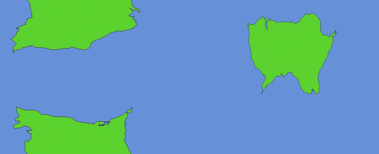
My first step was to make 2 fractal islands using the interactive programs from the aforementioned article. I took screenshots of each image and then placed them into one image, as seen below.

Note, I’m not sure the image needs such a rectangular aspect ratio. I tried this first and was pleased with the results and simply left it.

Next, I simply needed to wrap it around a 3D sphere set in space. Luckily, I’m familiar with POV-Ray, a free raytracing program. I used the following code, where my image was labeled planet2.jpg:


#include "colors.inc"
#include "stars.inc"

camera {
location <-1, 1.2, -6>
look_at <0,0,0>
angle 35
}

light_source { <500,500,-1000> White }
light_source { <-500,500,-1000> White }

sphere{<0,0,0>,1
pigment{
image_map {
jpeg "planet2.jpg"
map_type 1
interpolate 2
}
}
}

sphere {
<0, 0, 0>, 1
texture {Starfield1}
finish {ambient 1 diffuse 0}
scale 100000
}


So, how did I do? You judge for yourself. In fact, try it yourself and see if you can create a better image! You could remove the blue and replace it with a more realistic image of water. Or…If you give it a try, I’d enjoy seeing your planet!

Service-learning offers unique educational opportunities for students to apply their learning to issues of community interest. This post will discuss how I have integrated service-learning into a final project used in a discrete math modeling course. The course teaches such topics as Monte Carlo simulation, queuing theory, Markov Chains, and optimization. The capstone group project requires students to create a mathematical model for a problem posed by a local nonprofit organization. Topics included designing the layout of a parking lot for a local food pantry and assigning elementary students into practicum groups according to scheduling constraints and indicated interests for a local elementary school. The final model and recommendations from it were presented in a public poster session and in a paper.

Why use modeling in service-learning? The following quote from John von Neumann (a noted mathematician and computer scientist which is fitting given the ways this class integrates math and computing) motivates a reason:

If people do not believe that mathematics is simple, it is only because they do not realize how complicated life is.

Projects from the community that lend themselves to the discrete modeling topics of this course ideally contextualize learning math modeling. Why model? The world is often too complex to understand otherwise. Math modeling ideally can simplify a phenomenon and still capture its general behavior, offering analysis that is otherwise difficult if not impossible.

Seeing the role of modeling, I needed projects. At Davidson College, this is done with the aid of the Center for Civic Engagement. To aid that office in its call for proposals, I supplied examples of the types of problems my students study and solve. Such examples enable leaders in the non-profit organizations to think about their needs in relation to our skills. In the end, I need 6 projects for the class. Both years, I made personal contacts with organizations to create one or two projects that supplemented those submitted to the Center. Once the call is made, I receive the project proposals and in each case think about how I might tackle them. It should be noted that while I tell the students my ideas they are not bound to them.

After selecting the projects, I communicated with the community partners regarding follow up questions and the schedule (noting the weeks that students would want to meet and the time and date for the poster session). The email also thanked the partners for taking part in the educational process of the students. While the hope is that the students’ work would produce helpful and insightful results for the nonprofits, working on open-ended problems inherently involves unpredictable outcomes, which in itself is a unique and important learning environment for the students.

The students prepare for these final projects through the content learned through the course and a mid-semester project. The midterm project is similar although not set within a community-based problem. The earlier task requires working in a team of 3 on the Mathematical Content in Modeling (MCM) sponsored by COMAP. In 2011, three thousand teams participated from around the world. My students work on the discrete problem. The students’ success and fondness for these problems played an important role in my considering service-based problems as a final project.

In terms of content, the class introduces Monte Carlo simulation and queues. Simulation is often a tool employed on the MCM. They also learn Markov Chains which includes a discussion of PageRank (both as a simulation and as a Markov Chain). To see a way of introducing PageRank as a simulation and Markov Chain see my co-authored Loci article Google-opoly. Since Markov Chains can be solved using simulation, this technique, while important and useful, is rarely used on the MCM or final project. The last tool is linear programming. Students often use this on the final projects. A fun binary integer programming problem is applying such techniques to Sudoku. For a Loci article on this, see my co-authored article Integer Programming Model for the Sudoku Problem.

To begin the projects, I select teams. While students can request team members, I make the final decisions. Teams are assigned such that each group has a programmer and a writer. The last person is selected with mathematical diversity in mind. Generally, the groups work quite well together and such composition is helpful for the projects.

The teams are announced on a Monday. At the same time, I present all 6 projects and give a summary of how I would approach the problem. Again, many teams end up developing their own approaches. Still, my ideas serve as a helpful springboard for their work. The next day, a representative from each group submits their team’s ranking for all 6 problems. I assign projects to teams in the order the teams submit their rankings, which begin at an announced time. The first team gets their first choice. All remaining teams get their highest ranked problem that has not yet been assigned. The submissions are made online using a Blackboard discussion list. This enables me to set a specific time, like 10 AM, as the moment submissions will be accepted. From here the class follows this schedule

• Week 1 – Teams assigned, topics presented and assigned
• Week 2 – Proposal due – These are returned with comments by the next class period.
• Week 3 – Revised proposal due – Each proposal is edited with my comments in mind.
• Weeks 3 & 5 – A day of class is set aside for project meetings. If helpful, students can meet elsewhere during this time, which sometimes allows for a visit with the community partner.
• Week 6 – Poster session that the community partners attend along with members of the public and college community.
• Week 7 – Final paper is due. The paper includes an executive summary that is suitable for the community partner to read and know the recommendations of the group. The paper 8-10 pages (a maximum of 20 pages) includes the details and is what I read to assess their modeling techniques.

Here are two projects that give a sense as to their variety.

Community School of Davidson (CSD) – Assign students into practicum groups (where each group is capped at a maximum size that may vary from group to group). In particular, students fill out an application giving their top three choices for assignment.

For this problem, students used linear programming. The problem contains a lot of decision variables. As such, it couldn’t be solved using the Solver tool of Excel. Students decided to automate the process and use the NEO Server for Optimization.

Ada Jenkins Center – Design layout for the food pantry’s new location that will include walk in refrigeration units, shelves and storage.

The biggest part of this problem involved comparing configurations of shelving. The team created by horizontal and vertical configurations and compared their efficiency using both linear programming (for how items were shelved) and Monte Carlo simulation (for how people moved through the pantry). Below you see two of the layouts created by the team.

The team compared configurations, balancing amount of people serviced by layout with the amount of food stored, that also did and did not allow passing of the shopping carts used to collect the food. This, like the CSD project, was well received by the community partner. The ideas were used. With a few tweaks to student work, the pantry “managed to get approximately 40% more space in the new pantry and it is now possible for carts to pass in the aisles.”

The service-learning projects are as applied, in many ways, as applied math can be! The students get to see their gifts and knowledge of mathematics benefit the community. They leave their intellectual imprint on the community in which they lived for 4 years of college. The students reflect these types of insights in their comments in the student evaluations. Here are two:

“I thought the MCM and final project were awesome. Not only did I learn a great deal about how to write a math modeling paper but I also grew very close to my teammates. By the end of the term, I felt like the class was a family.”

“Best class I have had at Davidson; very interesting, good blend of concepts vs. real life application, challenging but fair, and a community project where we can actually see the results of our work.”

Interested in service-based projects? They can take many, many forms. This is the one that fit this course. Look up such ideas online, look for books on the topic, and envision how your class can engage with the community with their content.

Increasingly, I’ve been asked about my work with Amy Langville in sports ranking. In particular, students and faculty have been interested in researching or teaching ranking methods based in linear algebra. To help enable others tailor their work, I inevitably discuss how to find sports data. One of the easiest ways to explore existing methods is to apply them to online datasets. In this blog entry, I’ll explain how to access data that would enable one to rank the almost 350 Division I Men’s Basketball Teams. We’ve used such data to create math-generated brackets for March Madness.

Our task in sports ranking is straight forward. We need data. From this data, we rank the teams. We’ll see how to access season data for every game played by NCAA Division I Men’s basketball teams.

First, let’s understand how to interpret the data. One file will contain information on each game during the season. Each row of the file corresponds to a game and the columns contain the following data:

• column 1 = date of game as measured as days since 1/1/0000
• column 2 = date in YYYYMMDD format
• column 3 = team 1 index
• column 4 = team 1 score
• column 5 = team 1 home field (1 = home, -1 = away, 0 = neutral)
• column 6 = team 2 index
• column 7 = team 2 score
• column 8 = team 2 home field (1 = home, -1 = away, 0 = neutral)

For example, here are a few rows from games played in 2008.

733721, 20081110, 98, 65, 0, 114, 63, 0,
733721, 20081110, 75, 80, 1, 228, 49, -1,
733722, 20081111, 206, 73, 0, 128, 60, 0,
733722, 20081111, 114, 76, 0, 228, 57, 0,

We see from this data that on November 10, 2008 team 98 beat team 114 by the score of 64-63 on a neutral court. Also on that day, team 75 beat team 228 at home by a score 80-49. You should be able to read the remaining two rows of data extracted from the dataset.

Who’s who? Another data file indicates the correspondence between the natural numbers and teams. The first few rows again from 2008 are:

1, Air_Force
2, Akron
3, Alabama
4, Alabama_A&M
5, Alabama_St
6, Albany_NY
7, Alcorn_St
8, American_Univ
9, Appalachian_St

Now, we only need to download such datasets. Let’s download the data for the 2010-11 season. Here are the steps:

1. Visit http://www.masseyratings.com/data.php.
2. Scroll to the bottom and select Basketball > College Basketball > 2011
3. Click the cb2011 link at the top of the web page.
4. Navigate to NCAA > NCAA I > Scores
5. Visit the All link.
6. To download the game data, select the Intra and Matlab Games
7. To download the team data, select the Intra and Matlab Teams

Clearly, the data is Matlab-ready. Loading the games is quite easy. Here is the Matlab code I use:

fid = fopen(gameFilename);
gameData=load(gameFilename);
numberOfGames = size(gameData, 1);

Now, we have a matrix gameData that has each column of our
input file as a column in our matrix. So the input file:

733721, 20081110, 98, 65, 0, 114, 63, 0,
733721, 20081110, 75, 80, 1, 228, 49, -1,
733722, 20081111, 206, 73, 0, 128, 60, 0,
733722, 20081111, 114, 76, 0, 228, 57, 0,

becomes the matrix

Loading the team names is a bit more involved. Here is the code I use:

fid = fopen(teamFilename);
counter = 0;
while (ischar(teamname))
counter = counter + 1;
[token, remain] = strtok(teamname);
teamname = strtok(remain);
teamname=cellstr(teamname);
teamNames(counter) = teamname;
teamname = fgetl(fid);
end
fclose(fid);
numTeams = counter;

That’s it! Interested in another sport? Search around the Massey site and see what you find. If you can’t find it there, look around the Internet as you may find useful data elsewhere. Happy ranking!

Algebra covers solution techniques to solve linear systems like 2x – 3y = 5 and 3x + 2y = 1. Removing y, for instance, solving for x and then substituting the value for x to find y yields the solution x = 1 and y = -1.

Another way to represent the equations is as a matrix system, with its two unknowns x and y:

The matrix notation serves as useful bookkeeping, which will help us keep track as we form a larger linear system below.

Time for some linear thinking as we rank sports teams with the Colley method, which is a math technique used by the Bowl Championship Series, the organization that determines which college football teams are invited to which bowl games. The Colley method was created by astrophysicist Wesley Colley who saw problems with ranking by winning percentage and developed this method.

This blog entry will bypass the derivation of the method, although interesting, in order to focus on the mechanics of forming the associated linear system. This will enable us to focus on the ease and accessibility of the method. Interested in the derivation? Then, see the essay, Bracketology: How can math help?, from Math Awareness Month 2010. The article uses the Colley method to create personalized brackets for March Madness. The article also derives another technique used by the BCS called the Massey method and gives techniques that adapt each method to model momentum in a season.

In this article, we will focus on a fictional series of games within the South Division of the NFL. We’ll represent the records of the teams by a graph. An arrow from team A to team B indicates that team A beat team B in a game. So, we see below that the Panthers beat both the Buccaneers and the Falcons but did not even play the Saints. If you are unfamiliar with the teams then note that in clockwise order starting in the upper lefthand corner, the teams are the Saints, the Buccaneers, the Panthers and the Falcons.

First, we will form a matrix necessary to rank the teams. We’ll represent this matrix as a table. Each row of the table and each column corresponds to one of the teams. We have written the team’s name that is associated with each row and column in the table below.

	Saints	Buccaneers	Panthers	Falcons
Saints
Buccaneers
Panthers
Falcons

Now the question is what numbers to enter into the table.

For the entry in row 1 (Saints) and column 2 (Buccaneers), we put the number of times the two teams played multiplied by -1. Since the Saints and Buccaneers played once, we put -1. This is done in a similar way for all the entries except those on the diagonal. The entry in row 1 (Saints) and column 1 (Saints) equals the sum of 2 and the total number of games played by the Saints, which equals 4. Performing this task for all the teams creates the following table:

	Saints	Buccaneers	Panthers	Falcons
Saints	4	-1	0	-1
Buccaneers	-1	5	-1	-1
Panthers	0	-1	4	-1
Falcons	-1	-1	-1	5

Now, we have only to form the vector for the righthand side of the linear equation. Each row in that vector corresponds to the same team that it did in the matrix. So, row 1 in the vector associates with the Saints. Let W equal the number of wins by the Saints and L equal the number of losses. Then in the first row of the vector, we place the number 1 + 1/2(W – L). The Saints had 1 win and 1 loss so we place a 1 in that entry in the vector. Continuing in this way forms the vector:

In this way, we can express the linear system in matrix form as:

While a rather modest system compared to what we would use if we rated all the NFL teams, this system is still rather big for solving by hand. Given you are reading this blog, I’ll assume you have online access and can use WolframAlpha. WolframAlpha enables one to solve such systems. Here is the WolframAlpha entry that ranks the South Division of the NFL!

We that the solution is:

These are the ratings for the teams. The higher the rating, the better ranked the team. Therefore, the teams are ranked (from best to worst) Panthers, Saints and for a tie for third between the Buccaneers and Falcons.

This model would predict that the Panthers would easily beat any of the other three teams. Would that be the case? Should you book a flight to Vegas to play the odds? Keep in mind we have linear equations which means we are assuming life is linear. Just like the contour of the linemen, football is often not linear. A lot of variables beyond a win-loss record can play into a game. Perhaps one team plays better at home or a team struggles in the cold or….What then? Underneath this method is a model which can be altered but even so, it will be a model, which is intended to reflect but not exactly replicate life. So, give the NFL your best rating and still sit back and enjoy the games as you never know on any given Sunday what might happen!

As the fall semester of 2010 ended, I assigned a rather comical assignment in my Calculus 2 classes.

Students were told that the assignment was designed to aid in their preparations for the final exam. They could work with up to 2 other students. The assignment involved picking any content of the semester and create a cartoon. Along with the cartoon, students included a sentence indicating the content the drawing was intended to help someone learn and the corresponding section in the text.

For full credit, the cartoon

• had to be related to content from this semester of Calculus II material,
• could contain one panel or multiple panels, and
• could be drawn by hand or with a computer.

The cartoons were then used as we reviewed the semester’s material in preparation for the final.

To aid students concerned about their drawing skills, I demonstrated how to easily create a cartoon in PowerPoint. First, find a picture you like. For example, I entered “ski cartoon” into Google images and found the pictures of the fox and skier seen in the image below. Then, I simply pasted them into PowerPoint and used the drawing features to create the slope, speech bubble, words and surrounding panel. Here is my example:

A few days later, the classroom buzzed as students handed in their cartoons and shared them with each other often before submitting their assignment. I look forward to using the assignment again.

Enjoy the gallery of their work below.

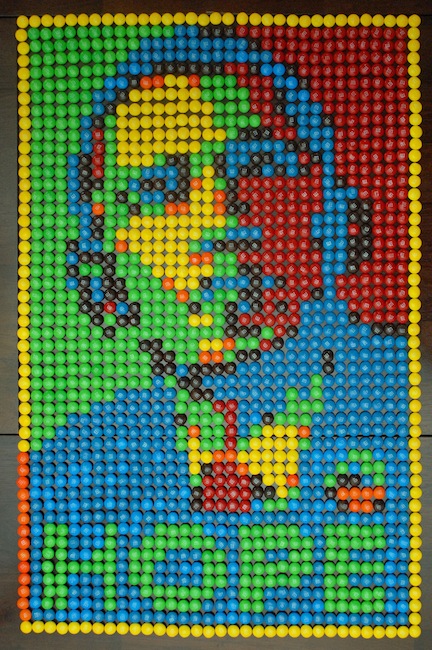
Let’s play with some food and create mosaics with pieces of candy. We need to place the treats so the resulting image will visually approximate an underlying picture. In this post, you’ll have the opportunity to create mosaics with a variety of candies. For now, we’ll use M&Ms. Fortunately, they melt in your mouth and not in your hand, giving us ample time to create our tiling. Our palette will be the colors from a standard bag of the M&Ms as seen below.

The image we want to approximate with a tiling will be called our target image. Let’s use the poster from the 2008 presidential election that depicted a stylized image of Barack Obama and became synonymous with the campaign.

Our tiles will replace square regions of our target image. For example, the image to the right is such a square region from the image above. This region is a collection of color pixels. Each pixel is represented as a coordinate triplet (r, g, b), where r is the amount of red, g is the amount of green and b is the amount of blue. For each square region, the average “color” is computed by averaging the red, blue and green intensities of each pixel in the region.

The color of M&Ms could be found in a similar way. Instead, we’ll take the color of an M&M to equal the color of a pixel within an image of an M&M with the same color.

Which M&M replaces a given square? The M&M with the “closest” color to the square of interest. For example, suppose the average color of a square region is (120.75, 40.25, 103.25). Let’s take the color of a blue and red M&M to be (0, 48, 106) and (202, 18, 44), respectively.

The distance between the average color and the blue M&M would be

The distance between the average color and a red M&M would be

So, between a blue and red M&M, we choose the red M&M.

How does such a method do in constructing a mosaic? Recognize the mosaic below?

What if we use more or less M&Ms? What if we try a different target image? What happens with other types of candy?

What if we use more or less M&Ms? What if we try a different target image? What happens with other types of candy? Click the image below to visit a webpage that contains an applet to let you explore such questions!

Once you’ve created an image you like, go and buy a bag (maybe several) of M&Ms, Jelly Bellies, Kisses, Peeps or Gummy Bears and make your mosaic by hand!

The best part is taking it apart!

The Traveling Salesman Problem (TSP) is an NP-hard problem in combinatorial optimization. Given a list of cities and the distance between each pair of cities, the TSP requires finding a shortest possible tour that visits each city exactly once and returns to the starting point. The TSP is one of the most intensely studied problems in computational math. For an extensive resource regarding history, applications and research of the TSP, see Traveling Salesman Problem.

The TSP increases in difficulty as the number of cities grows. This is connected to the computational difficulty of the problem. For instance, solving a TSP with 30 cities would be very difficult by hand. For instance, in 1962, Proctor and Gamble ran a contest that required solving a TSP on 33 cities. The poster is seen to the right. More than one person submitted an optimal value and among them was an early TSP researcher, Professor Gerald Thompson of Carnegie Mellon University.

A group in my discrete math modeling class is working on a TSP-like problem for a non-profit organization. They are wanting to recommend carpool groups to families whose children attend a local school. An important part of the problem is acquiring the pairwise costs of traveling between two homes. This could be distance or possibly time, as sometimes distance isn’t an accurate measure of the cost since we often want to minimize driving time.

The group found the Google API and requested help in pulling driving distances from Google for known locations. As I read the documentation, I began fiddling with MATLAB code and in the end had a working program. Thinking this might be helpful to others, I decided to create a function getGoogleMap.m that grabs the driving distance and time from Google between two inputted addresses. Then, I created a driver googleTable.m that creates a city by city table of distances and times between locations. The code creates the tables in text and in HTML.

As I experimented with the code, I used the following locations: the Space Needle, the Empire State Building, Davidson College, the Alamo, and the Hollywood sign, which were numbered 1 to 5, respectively. You can also see the locations and their numbers in the picture above. This code creates the following tables, again produced in HTML by the MATLAB code. I simply pasted the resulting HTML into this blog.

DISTANCES (in miles)
	City 1	City 2	City 3	City 4	City 5
City 1	0.0	2855.8	2765.2	2163.8	1130.1
City 2	2855.8	0.0	627.7	1826.6	2809.7
City 3	2765.2	627.7	0.0	1244.9	2427.3
City 4	2163.8	1826.6	1244.9	0.0	1361.6
City 5	1130.1	2809.7	2427.3	1361.6	0.0

Again, I also inputted times between locations as distance isn’t always the best measure of the length of a trip.

TIMES
	City 1	City 2	City 3	City 4	City 5
City 1	0 min	46 hr, 31 min	44 hr, 49 min	36 hr, 22 min	18 hr, 39 min
City 2	46 hr, 31 min	0 min	10 hr, 20 min	29 hr, 32 min	44 hr, 52 min
City 3	44 hr, 49 min	10 hr, 20 min	0 min	20 hr, 12 min	38 hr, 12 min
City 4	36 hr, 22 min	29 hr, 32 min	20 hr, 12 min	0 min	21 hr, 21 min
City 5	18 hr, 39 min	44 hr, 52 min	38 hr, 12 min	21 hr, 21 min	0 min

Ironically, I’m discussing the TSP in modeling today. The code was developed for my students but will soon play a role in my teaching.

I’ll leave you with a popular teaser that I use in class. Sometimes, seeing that something can be formulated as a TSP or TSP-like is a key observation in modeling. Consider the following game from http://archive.ite.journal.informs.org/Vol3No1/Chlond/Touching.htm.

In the start position above zero touches 2 squares from other numbers, 1 touches 3 squares from other numbers, 2 touches 4 squares from other numbers, and so on to 9, which touches 4 squares from other numbers. If you multiplied each number by the number of squares it touched, and summed the result, you get

0(2) + 1(3) + 2(4) + 3(6) + 4(7) + 5(8) + 6(5) + 7(6) + 8(9) + 9(4) = 277

Can you find a lower value? What configuration leads to the lowest possible value? Click the link above for an applet that let’s you try. Further, how is this like a TSP? One change to the game will make it a TSP! How? Why? That’s the tease in the teaser!

Beware – the game can be a bit addictive!